Spark

Theory

Spark vs MapReduce

Spark is a general purpose engine for parallel data processing.

When I first heard about Spark I was already familiar with MapReduce, so it’s useful to clear up the differences between the two.

Like MapReduce it can be used for batch data processing in parallel. But it’s much faster. To see why, consider the life of a MapReduce job:

Read data from disk -> Map data -> Reduce data -> Write data to disk

Now, what if you want to run another MapReduce job which operates on the output of that job? The process would then be:

(Read data from disk -> Map data -> Reduce data -> Write data to disk) --> (Read data from disk -> Map data -> Reduce data -> Write data to disk)

See the problem? Data is being written to disk after each job, and disk I/O is expensive. In addition a JVM is started for each job which has significant overhead.

Spark solves this problem. It allows you keep datasets in memory between processing stages, allowing arbitrary data processing pipelines to be executed without writing to disk (if you have enough RAM 😉).

Another benefit of Spark is that it abstracts parallelism away from the developer. This means much simpler APIs which aren’t confined by the map reduce programming model.

Because data is kept in memory and the APIs are so simple, Spark is ripe for interactive data analysis. You can run Spark code using a REPL or notebooks as if you were analysing data on your local machine 😍

It’s not just simplicity and speed. Spark has become more popular than MapReduce for other reasons too:

• There are APIs for other types of data processing - graph, streaming, machine learning etc.
• APIs are available in a number of languages: Scala, Python, Java and R. I’ll use Scala for all examples.

APIs

There are a few Spark APIs to choose from.

RDDs

The Resilient Distributed Dataset (RDD) is a read-only, partitioned collection of records that can be operated on in parallel.

It is the most basic data abstraction available.

You can create an RDD by:

1. Reading from a file (e.g. text file, HDFS file)
2. Parallelising a scala collection (e.g. List)
3. Transforming an existing RDD

Once you’ve created an RDD, there are a two types of operations you can perform:

1. Transformation: Manipulate an existing RDD to create a new one e.g. dataset.filter()
2. Action: Do something with the RDD e.g. dataset.count()

A few more importatnt points on RDDs:

• They’re evaluated lazily - they’re computed when an action is performed.
• They’re fault tolerant. This is achieved by storing RDD lineage. That way in the event of an error, the RDD can be recomputed.
• The RDD API is accessed through the SparkContext class, while the Dataframe and Dataset APIs are accessed through the SparkSession class.

RDDs are very flexible and provide useful functional transformations. However, they don’t provide a mechanism for specifying a data schema which means the operations are quite low level. This issue is resolved by the newer APIs.

Dataframes

Dataframes are similar to RDDs but they take into account the schema of the data. Using this schema data is organised into rows and columns - it’s tabular. This makes dataframes suitable for processing structured data.

Having a structure facilitates higher levels of abstraction and, consequently, an even more user-friendly API. So user friendly that you can even use plain SQL to manipulate dataframes.

Additionally, dataframes are part of the spark-sql package and utilise the Catalyst optimizer to build relational query plans. This makes Dataframe operations more efficient than RDD operations.

With the introduction of Datasets, a DataFrame is simply a Dataset[Row].

Datasets

Dataframes are great but they aren’t type safe. To understand what this means, consider the following csv file:

Item,Price
Apples,3.5
Oranges,4
Bananas,2

Say we want to get all the items with a price greater than 2:

val pricedf = spark.read
    .format("csv")
    .option("header","true")
    .option("inferSchema","true")
    .load("prices.csv")
pricedf.filter("price > 2").show

See the “price > 2” bit? Any error caused by this (e.g. the price column not existing, the operation not being valid for the price column’s data type etc.) won’t be caught until run time. Using datasets, you can catch ther errors at compile time:

case class Price(item:String, price:Double)
val priceds = spark.read
    .format("csv")
    .option("header","true")
    .option("inferSchema","true")
    .load("prices.csv")
    .as[Price]
priceds.filter(_.price > 2)

.as[Price] converts Dataset[Row] to Dataset[Price], which provides type safety as you can see in the line that follows it. You can see the full code highlighting this difference here.

Using Datasets does incur a slight performance cost as Spark’s internal representation of the rows need to be converted to JVM representations.

Note the Dataset API isn’t provided in Python as it’s a dynamically typed language (compile time type checking isn’t a thing).

Caching

Datasets are evaluated every time an action is performed on them, even if they have been accessed previously. To avoid this unnecessary computation the dataset can be cached by calling ds.cache(). It’s important to do this when the same data will be repeatedly accessed e.g. interactive analysis.

What happens if the dataset doesn’t fit in memory? Should you then spill to disk? Should you compress the data so it does fit?

For RDDs, the default cache storage level is MEMORY_ONLY. This means that partitions which can’t fit in memory will be recomputed. For Datasets, it’s MEMORY_AND_DISK. This means partitions that don’t fit in memory are spilled to disk.

You can override these defaults with persist(), which takes a number of storage levels. See the docs.

Cluster Managers

Spark applications run on a cluster with the following architecture:

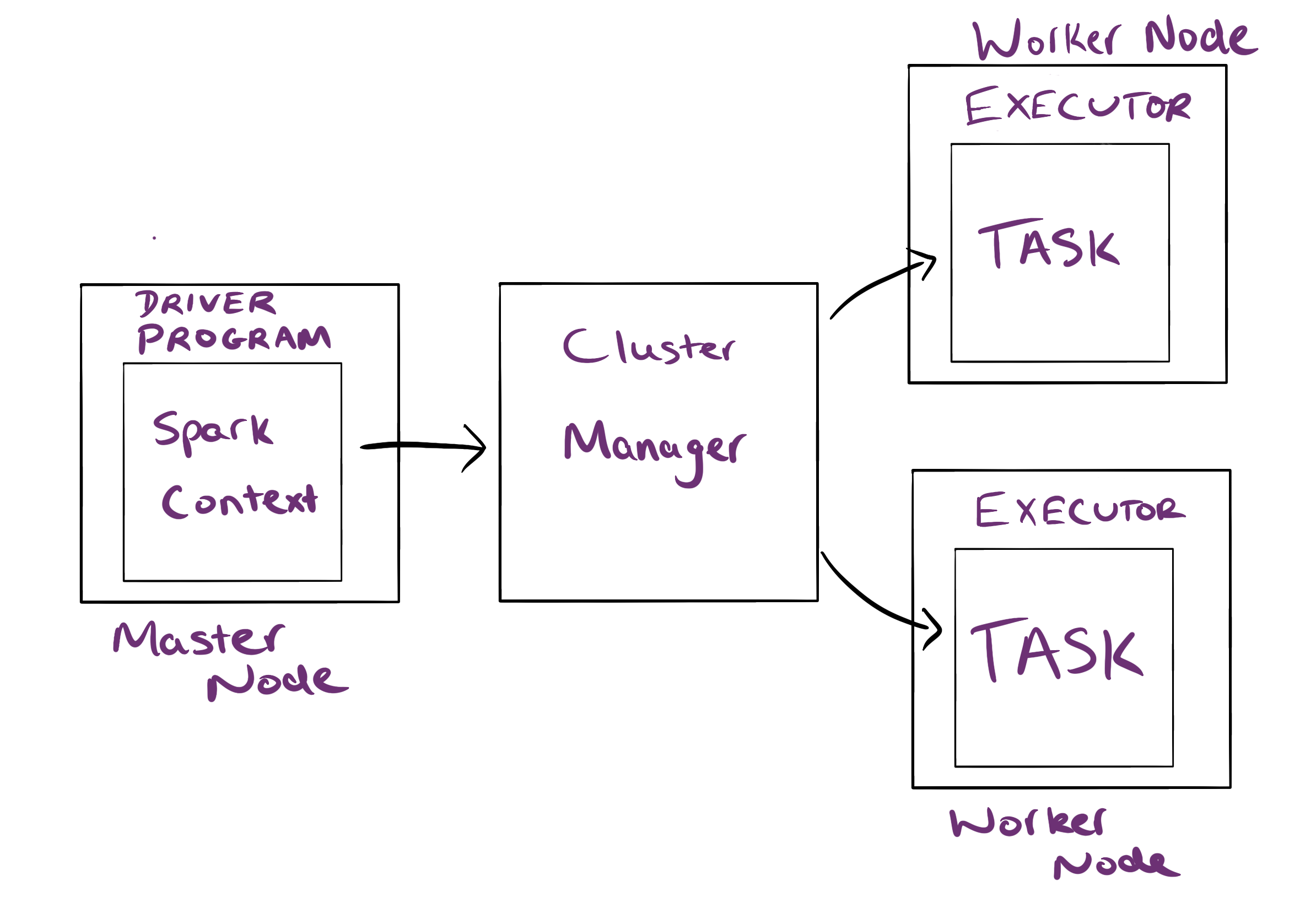
The worker nodes have a simple job - run tasks. These tasks are run on executors that are exclusive to the applications. The driver program schedules the tasks to be run.

There are many options for the cluster manager:

1. Standalone
2. Apache Mesos
3. YARN
4. Kubernetes

In addition Spark can also be run locally, where a single executor is running in the same JVM as the driver.

The cluster manager is specified by the --master option in the spark-submit command, which is used for submitting Spark applications.

There are two different application deployment modes that can be used with the cluster managers:

1. Client: The driver program is launched outside the cluster (on the machine that submitted the job). This is suitable for interactive analysis however, if the client goes down the application will fail.
2. Cluster: The driver program is launched within the cluster. This is suitable for long running jobs.

Stages and Tasks

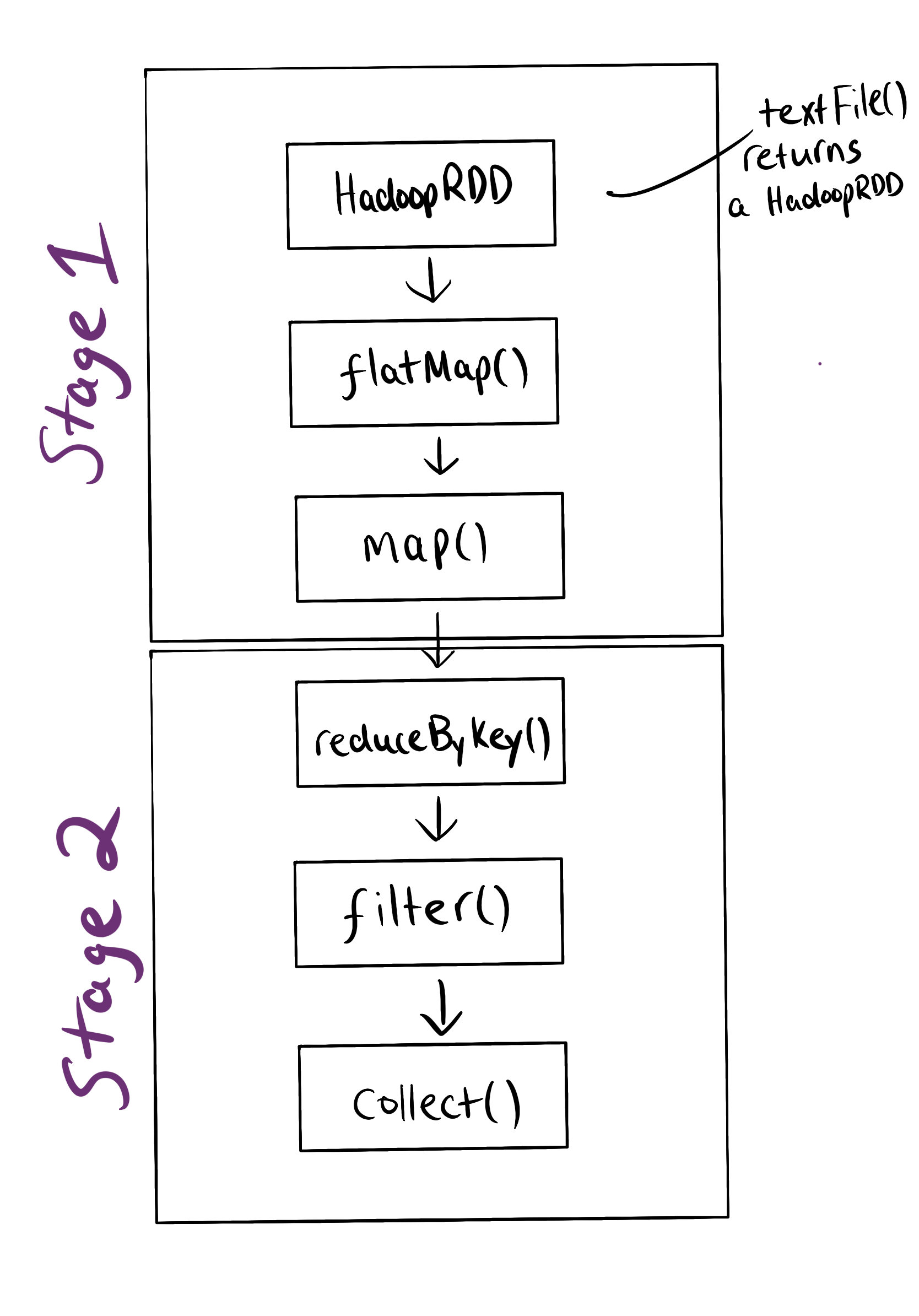
Each time an action is invoked on an RDD a job will run. This job is broken into stages using the RDD lineage. Stages are further broken down into tasks. To understand this consider the following piece of code which will show the words in a text file which appear at least twice:

val wordsAppearingTwice = sc.textFile(path)
      .flatMap(line => line.split(" "))
      .map(word => (word, 1))
      .reduceByKey(_+_)
      .filter(tuple => tuple._2 >= 2)
      .collect()

collect() is the action that causes the job to be submitted. The DAG scheduler then breaks the job into stages:

If you’re running this, you can use the toDebugString see it:

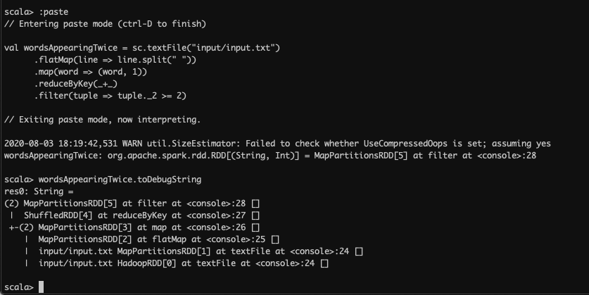
This execution plan is in the form of a directed acyclical graph (DAG), which is simply a directed graph with no cycles.

What determines the stage boundary? A stage is a pipeline of transformations which can be executed without shuffling data. Remember from MapReduce that the shuffle operation repartitions data. This will usually involve moving it between nodes, which is expensive.

The reduceByKey() operation does a shuffle. Why? All records ((word,1) pairs) with the same key need to be on the same partition to get one result per key.

Transformations that require a shuffle such as reduceByKey() are known as wide transformations, while those that don’t are known as narrow.

The execution plan will then be given to the task scheduler to break into tasks:

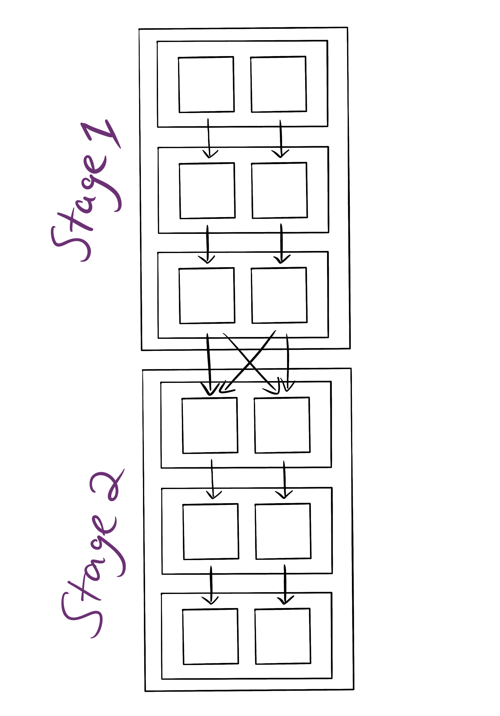
Note the number of tasks run for each step is determined by the number of partitions. In this case I’ve assumed the text file is stored in two partitions. You can repartition data arbitrarily using repartition(). It’s a good idea to do this if you are have too few partitions (not enough parallelism) or too many (too much overhead).

The tasks will then be run on executors. For more details check out this vid.

Web Interface

The Spark web interface runs on port 4040 however, it is only available for the duration of the application. When multiple apps are running, interfaces will be hosted on successively higher ports (4041, 4042 etc.).

To makes logs available at all times a history server needs to be run.

Local Examples

Installation

First install sbt. The instructions from the official documentation worked for me:

echo "deb https://dl.bintray.com/sbt/debian /" | sudo tee -a /etc/apt/sources.list.d/sbt.list
curl -sL "https://keyserver.ubuntu.com/pks/lookup?op=get&search=0x2EE0EA64E40A89B84B2DF73499E82A75642AC823" | sudo apt-key add
sudo apt-get update
sudo apt-get install sbt

Check it worked by running sbt --version.

Now install Spark:

1. Download the Spark tarball: curl -L -O http://spark_tarball_url. The url of the desired version can be found on the Spark downloads page.
2. Unpack it:

   sudo tar xzvf spark-*.tgz -C /opt
   cd /opt
   sudo mv spark-* spark
   

3. Update environment variables in your bash profile:

   export SPARK_HOME=/opt/spark
   export PATH=$PATH:$SPARK_HOME/bin
   

4. Check that was successful by running spark-shell --version

Shell Examples

Let’s create a WordCount program using the RDD API. First create the file to count and start spark shell:

echo "one\ntwo\none" > input.txt
spark-shell

Now count the words. To paste the following code into the shell type :paste, paste it and then ctrl-D.

val wordCounts = sc.textFile("input.txt")
    .flatMap(_.split(" ")) // split the collection of lines into a collection of words
    .map((_, 1))           // turn the collection of words into a collection of (word,1)
    .reduceByKey(_+_)      // count the occurrences of each word

// print out the resulting rdd
wordCounts.collect.foreach(println)

We could then write the final RDD back to disk as MapReduce does:

wordCounts.coalesce(1).saveAsTextFile("counted")

coalesce(1) function will simply move the data into one partition. The file will now be at ./counted/part-00000.

Submit Examples

This program can also be packaged as a Spark app. I’ve put this in a separate repository. You can run it as follows:

git clone https://github.com/jdoldissen/spark-word-count.git
cd spark-word-count
sbt package
spark-submit --class "wordcount.WordCountRDD" --master local target/scala-2.11/word-count-app_2.11-1.0.jar data/input.txt

Note data/input.txt is a parameter to the program.

If you’d like to see the code being run, it’s in src/main/scala/wordcount/WordCountRDD.scala.

Avocado Prices

Now let’s take a look at the dataset API. To do this we’ll analyse an avocado price dataset from Kaggle. Start spark-shell and then run the following commands:

// change "avocado.csv" to the path to your avocado dataset
val avdf = spark.read
    .format("csv")
    .option("header","true")
    .option("inferSchema","true")
    .load("avocado.csv")

avdf.cache()                                            // we'll be using the dataframe a lot, so let's cache it
avdf.show                                               // take a look to get an understanding of the data
avdf.printSchema                                        // have a look at the schema
avdf.select("region").distinct.count                    // get number of regions in the dataset
avdf.select(min("date")).show()                         // get date observations started
avdf.select(max("date")).show()                         // get date observations ended
avdf.orderBy(desc("averageprice")).limit(1).show        // show the row with the max avg price
avdf.orderBy(asc("averageprice")).limit(1).show         // show the row with the min avg price

As you can see, the highest avocado prices recorded were San Francisco’s organic avs in 2016. Let’s see if prices have dropped in recent times there:

avdf.filter("region = 'SanFrancisco'").orderBy(desc("date")).limit(2).show

By March 2018 the organic price had dropped to 1.64 - much better. What about price spikes in other regions? Let’s have a look at when each region had its highest price:

val maxprices = avdf
    .groupBy($"region".alias("max_region"))
    .agg(max("averageprice").alias("max_avg"))

avdf.join(
        maxprices, 
        avdf("region") === maxprices("max_region") && avdf("averageprice") === maxprices("max_avg")
    ).select("region","date","max_avg")
    .orderBy(desc("max_avg"))
    .show

Not the use of $ before the column name. That will convert region to Column("region"), which allows use to use functions like alias(). You don’t always have to use the dollar as you saw in the previous examples - most functions accept strings or columns.

The dataset queries mostly mirror SQL. In fact, you can even directly use SQL. For example to get the number of regsions in the dataframe:

avdf.createOrReplaceTempView("avprices")
spark.sql("SELECT COUNT(DISTINCT region) AS region_count FROM avprices").show

There’s a ton more you can do - see the docs for ideas.

Cluster Examples

Setup

It’s not too much extra work to run Spark with the YARN cluster manager, assuming you already have a Hadoop cluster. For instructions on how to set that up on a Raspberry Pi, see hadoop.

1. Add the following to you bash profile:

   export HADOOP_CONF_DIR=$HADOOP_HOME/etc/hadoop
   export LD_LIBRARY_PATH=$HADOOP_HOME/lib/native:$LD_LIBRARY_PATH
   

2. Open $SPARK_HOME/conf/spark-defaults.conf and add the following:

   spark.master            yarn
   spark.driver.memory     512m
   spark.yarn.am.memory    512m
   spark.executor.memory   512m
   

   Note this is setting memory allocation, which is dependent on available RAM.

3. Test Spark:

   start-all.sh
   spark-submit --master yarn --deploy-mode client --class org.apache.spark.examples.SparkPi $SPARK_HOME/examples/jars/spark-examples_2.11-x.y.z.jar 10
   

   You should see Pi is roughly 3.141843141843142 a few lines up from the end of the output.

Shell Examples

To load the avocado dataset used in the previous section from hdfs:

hadoop fs -mkdir csv 
hadoop fs -copyFromLocal avocado.csv csv/avocado.csv 
spark-shell --master yarn --deploy-mode client
val avdf = spark.read
    .format("csv")
    .option("header","true")
    .option("inferSchema","true")
    .load("hdfs:/user/pi/csv/avocado.csv")

You could also specify the namenode address in the hdfs path e.g. load(hdfs://pi1:9000/user/pi/csv/avocado.csv).

The normal dataframe commands can then be used.

Submit Examples

We can run a custom word count jar in a similar way to the previous section. First copy some words to count to hdfs (or just use an existing file):

echo "one\ntwo\none" > ~/hadoop-test/input/input.txt
hadoop fs -copyFromLocal ~/hadoop-test/input/input.txt input/input.txt

Now run the jar:

spark-submit --master yarn --deploy-mode client --class "wordcount.WordCountRDD" --master yarn target/scala-2.11/word-count-app_2.11-1.0.jar hdfs:/user/pi/input/input.txt

History Server

The Spark UI is only available while the job is running. To get logs afterwards, the history server must be running. To do this first add the following to $SPARK_HOME/conf/spark-defaults.conf:

spark.eventLog.enabled            true
spark.eventLog.dir                hdfs://<insert_master>:9000/spark-logs
spark.history.fs.logDirectory     hdfs://<insert_master>:9000/spark-logs

Then create the logs directory and start the server:

hadoop fs -mkdir /spark-logs
$SPARK_HOME/sbin/start-history-server.sh

Now after running a Spark job, go to http://<insert_master>:18080 to view the logs. You can also periodically clean up the logs:

spark.history.fs.cleaner.enabled  true
spark.history.fs.cleaner.interval 1d
spark.history.fs.cleaner.maxAge   7d